
Case study:
Fitting data to the Ideal Gas Law
A recent consulting customer had an interesting “regression-like” problem that didn’t fit neatly into a classical regression model. He receives small gas-filled vials, with different amounts of gas inside. He determines the quantity of gas — starting pressure and starting volume — by puncturing the vial, letting the gas expand into a series of evacuated chambers of known volume, and measuring the observed pressures.
![[diagram of apparatus]](ideal_fig1.png)
The Ideal Gas Law tells that, provided we keep the experiment at constant temperature, pressure and volume are inversely related. If we expand a sample of gas from volume V1 to volume V2, P1 x V1 = P2 x V2, or, rearranging the equation, the new pressure P2 = P1 / (V2/V1). If we knew the starting volume of gas, this would be a very simple linear regression problem: (P1, 1/V1), (P2, 1/V2), and so on would all lie on a straight line passing through the origin.
However, my customer didn’t know what his starting volume was. He only knew the volumes of the chambers into which he expanded the unknown amount of gas. So a typical data set from his laboratory looked like this:
| Expansion # | Pressure (bars) | Volume (cc) |
|---|---|---|
| 1 (unobservable) | P1 | V1 |
| 2 | P2=1.14 | V2=V1+40 |
| 3 | P3=0.61 | V3=V1+100 |
| 4 | P4=0.33 | V4=V1+200 |
| 5 | P5=0.15 | V5=V1+500 |
If I knew what V1 was, I would proceed by plotting (P2, 1/V2), (P3, 1/V3), (P4, 1/V4), and (P5, 1/V5), finding the line of best fit through those 4 points, and then calculating what P1 corresponded to 1/V1 on that line. But I don’t.
If I only had pencil-and-paper methods at my disposal, I could do something like find the value of V1 which caused those four points to lie on the straightest line, find that straightest line, and then estimate what P1 corresponded to 1/V1 on that line.
That method has two flaws. One is the inelegance of estimating the two unknowns one at a time, rather than simultaneously. Another, more serious, problem is that “find the straightest line” (find the set of points which maximizes r2) ignores the error structure of the observations. We know, from the manufacturer’s data on the pressure gauge, how much error to expect in the pressure measurements. We can ask our customer how carefully he calibrated the volumes of the four additional chambers.
Suppose that each of the four pressure measurements has an uncertainty of ±.01 bar. That means, in relative terms, Measurement 2 is almost ten times as precise as Measurement 5 is, and should be accorded more weight in determining what P1 and V1 were.
Writing and maximizing a likelihood function
A likelihood function is a tool for assessing how well a particular model fits a data set. We imagine that we know the unknown parameters — here, V1 and P1 — and then we suppose that our observations differ from the true pressures only due to measurement error. If we assume that the Vi are determined on the laboratory bench so well that there error is negligible, and each of the Pi suffers an error which is normally distributed with mean 0 and standard deviation .01 bar, then, recalling that the pdf of a normal distribution is FindMinimum[lik[k, vp], {k, vp}]
{0.624864, {k -> 77.1062, vp -> 27.5853}}
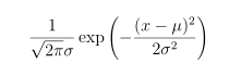
our likelihood function is the product of the probabilities of our four observations:
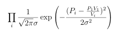
Usually we find it more convenient to take the logarithm of this, working with the log-likelihood:
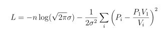
and we use the numerical optimizer of our choice to find
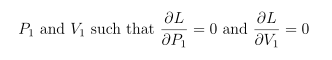
I chose to do it in Mathematica, and ran a block of code like the following to get my estimates for P1 and V1:
(* Test case: 25 cm^3 at 3 bar, expanded into 40/100/200/500 cm^3 *)
data = {{40, 1.14}, {100, .61}, {200, .33}, {500, .15}};
sterrs = {.01, .01, .01, .01}; (* SE of pressure measurements *)
n = Length[data];
lik[k_, vp_] :=
Sum[(data[[i, 2]] - k/(data[[i, 1]] + vp))^2/2/sterrs[[i]]^2, {i, n}]
(I used k=nRT for the total quantity of gas present, such that PiVi=k for every observation.) One of many nice statistical properties of maximum likelihood estimates is that for any maximum likelihood estimation, the variance-covariance matrix of the estimates can be found by inverting the Hessian (matrix of second partial derivatives of the log-likelihood): {{4.10888, 3.89867}, {3.89867, 4.02199}}
hessian = {{ D[lik[k, vp], {k, 2}],
D[D[lik[k, vp], k], vp]} ,
{D[D[lik[k, vp], k], vp],
D[lik[k, vp], {vp, 2}]}};
Inverse[hessian /. {k -> 77.1062, vp -> 27.5853} ]
This enables us to give an answer to our customer’s original question: our best estimate of k=PV is 77.11±2.03; our best estimate of V1, 27.59±2.01 cm3, and, combining these two, our best estimate of P1, 2.80±0.22 bar. (The data set used for this example was actually contructed by setting P1=25 cm3 and V1=3 bar, and then randomly perturbing and rounding off the expected pressures 1.153, 0.600, 0.333, and 0.143 bar.)
How is this better than what a physicist would do without a statistician’s help?
It’s possible to directly use any pair of observations to estimate P1 and V1. Using observations 2 and 3 for instance:
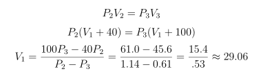
And, using the classical method for propagation of errors:
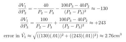
The physicist could repeat this calculation on each pair of his original measurements:
- 2 and 3: 29.06±2.76 cm3
- 2 and 4: 25.19±2.81 cm3
- 2 and 5: 29.67±5.40 cm3
- 3 and 4: 17.9±11.2 cm3
- 3 and 5: 33.6±11.9 cm3
- 4 and 5: 50.0±33.6 cm3
How is he supposed to combine those 6 non-independent estimates of V1 into something sensible? Perhaps a weighted average. (And if you choose weights inversely proportional to the variances, you’ll come up with a pooled estimate of 27.41±2.91 cm3.) It takes a lot of tedious calculations, not reproduced here, to get a shaky and somewhat difficult-to-defend final answer.
The maximum likelihood approach is easier to justify theoretically and easier to explain to a layman, as well as providing a clearer picture of how the uncertainty in the pressure measurements P2-P5 translates into uncertainty in the estimated volume V1. Not to mention — if you aren’t afraid of numerical maximization, it is a lot less work!
Contact us if you have a model fitting problem that doesn’t fit comfortably into a textbook regression model. Large or small, one variable or many, we can set up a likelihood equation for you and calculate MLEs for you.
Back to maximum likelihood page
Back to main optimization page